
HGS RESEARCH HIGHLIGHT – Evaluation of Hydraulic Conductivity Estimates from Various Approaches with Groundwater Flow Models

Sun, D., Luo, N., Vandenhoff, A., McCall, W., Zhao, Z., Wang, C., Rudolph, D. L., & Illman, W. A. (2023). Evaluation of Hydraulic Conductivity Estimates from Various Approaches with Groundwater Flow Models. In Groundwater. Wiley. https://doi.org/10.1111/gwat.13348
“A question frequently encountered by hydrogeologists is what approach should be adopted to obtain K estimates at a given site for groundwater modeling?[...]The main objective of this study is to evaluate various K estimates from three categories of site characterization methods
[...]
[T]he performance of each approach is first qualitatively analyzed by comparing K estimates to site geology. Then, we quantitatively evaluate the K estimates
[...]
[A] three-dimensional (3D) forward groundwater model is developed using HydroGeoSphere (HGS) (Aquanty 2019) for forward simulations of steady-state drawdown data from seven independent pumping tests[...]”

Fig. 2. Cross-sectional view of the 19-layer geological zonation model with CMT and PW screened intervals shown in cross sections C-C′ and D-D′. Cross sections along A-A′ and B-B′ are available in Figure S1. The 19 layers represent 7 different material types as indicated in the stratigraphic index. The 7 material types were obtained through examination of cores from 18 boreholes at the site. Specifically, the 19 layers indicated on cross sections C-C′ and D-D′ are clay (1, 4, 8, 12, 16, 18), silt and clay (17, 19), silt (2, 7, 10, 14), sandy silt (6, 9, 13), silt and sand (5), sand (3, 11), and sand and gravel (15). On cross sections C-C′ and D-D′, layer numbers are italicized and numbers along PW and CMT wells indicate port numbers (e.g., PW1-1, PW1-2, and so on).
A new study by researchers at the University of Waterloo, Chinese Academy of Sciences and Geoprobe Systems Inc. utilized HydroGeoSphere to evaluate estimates of hydraulic conductivity produced using a variety of techniques.
Over several decades a wide variety of techniques have been used to estimate the hydraulic flow properties of the subsurface. Here the authors have produced heterogeneous hydraulic conductivity (K) distributions at a heavily instrumented research site using 6 distinct techniques (slight variations in some tests resulted in 9 distinct K distributions):
1a) Grain size analysis using three empirical models
1b) Lab-based Permeameter Tests of repacked samples
1c) Slug Tests performed at 7 intervals each across four monitoring wells
2a-c) Hydraulic Profiling Tool (HPT) tests (evaluated using 3 different formulae)
3a) Inverse modelling and parameter estimation using a PEST Calibrated Geologic Model
3b-c) Transient Hydraulic Tomography (THT) (with average and high levels of parameterization)
Which of these techniques is the best, and how do the resulting K distributions compare to each other? Well… it might be impossible to say which technique is “best” considering the highly-heterogeneous nature of the subsurface and the unique nature of each site (not to mention practical considerations like cost).
But in this study the authors evaluated the performance of the various K distribution maps by applying them to a highly refined HydroGeoSphere model. The HGS models were then used to reproduce drawdown from seven pumping/injection tests (these 7 tests were distinct from any tests used to produce K distribution maps) under both steady-state and transient conditions.
Overall conclusions of this study (for this particular site) indicate that K distributions from conventional methods (1a-c) and HPT testing (2a-c) produce biased results under both steady-state and transient conditions (i.e. overestimating drawdown), and that the inverse modelling approaches (3a-c, especially the highly parameterized THT test) yielded the best predictions of drawdown under both steady-state and transient conditions.
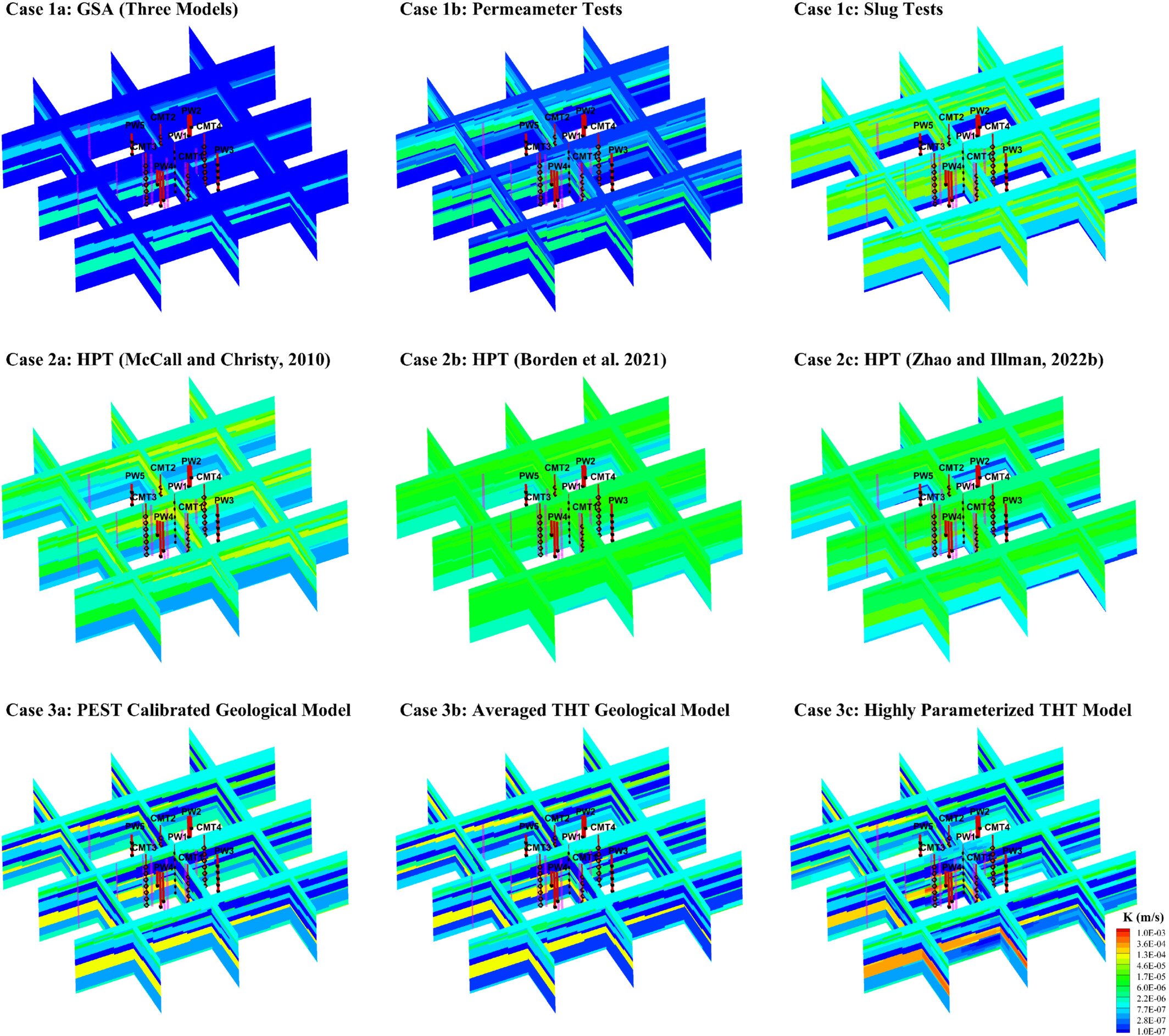
Fig. 6. K distributions at the NCRS from various site characterization approaches. CMT and PW well locations (red lines) along with their screened intervals (black color) as well as HPT survey locations (dashed pink lines) are shown on each subfigure.
Abstract:
Significant efforts have been expended for improved characterization of hydraulic conductivity (K) and specific storage (Ss) to better understand groundwater flow and contaminant transport processes. Conventional methods including grain size analyses (GSA), permeameter, slug, and pumping tests have been utilized extensively, while Direct Push-based Hydraulic Profiling Tool (HPT) surveys have been developed to obtain high-resolution K estimates. Moreover, inverse modeling approaches based on geology-based zonations, and highly parameterized Hydraulic Tomography (HT) have also been advanced to map spatial variations of K and Ss between and beyond boreholes. While different methods are available, it is unclear which one yields K estimates that are most useful for high resolution predictions of groundwater flow. Therefore, the main objective of this study is to evaluate various K estimates at a highly heterogeneous field site obtained with three categories of characterization techniques including: (1) conventional methods (GSA, permeameter, and slug tests); (2) HPT surveys; and (3) inverse modeling based on geology-based zonations and highly parameterized approaches. The performance of each approach is first qualitatively analyzed by comparing K estimates to site geology. Then, steady-state and transient groundwater flow models are employed to quantitatively assess various K estimates by simulating pumping tests not used for parameter estimation. Results reveal that inverse modeling approaches yield the best drawdown predictions under both steady and transient conditions. In contrast, conventional methods and HPT surveys yield biased predictions. Based on our research, it appears that inverse modeling and data fusion are necessary steps in predicting accurate groundwater flow behavior.
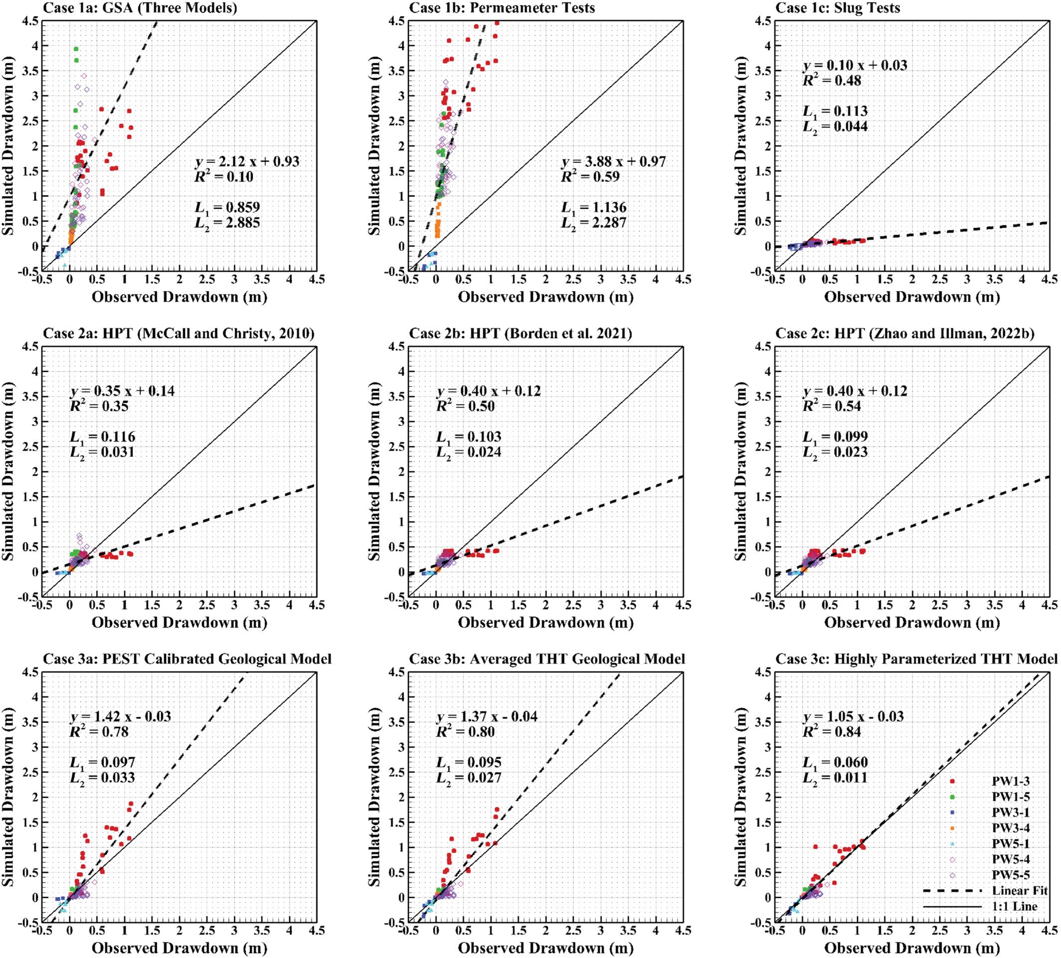
Fig. 7. Scatterplots of observed versus simulated drawdowns from various K characterization approaches for model validation under steady state conditions.

Fig 8. Scatterplots of observed versus simulated drawdowns from various K characterization approaches for model validation under transient conditions.
Want to learn more about Transient Hydraulic Tomography (THT) analysis for the estimation of hydraulic conductivity (K) and specific storage (Ss)? Here’s a related research highlight: Hydraulic tomography analysis of municipal-well operation data with geology-based groundwater models