
HGS RESEARCH HIGHLIGHT - Simulating seasonal variations of tile drainage discharge in an agricultural catchment

De Schepper, G., Therrien, R., Refsgaard, J. C., He, X., Kjaergaard, C., & Iversen, B. V. (2017). Simulating seasonal variations of tile drainage discharge in an agricultural catchment. In Water Resources Research (Vol. 53, Issue 5, pp. 3896–3920). American Geophysical Union (AGU). https://doi.org/10.1002/2016wr020209
“Results indicate that, while both models (HydroGeoSphere and Mike SHE) provide realistic simulations of drainage dynamics at the catchment scale (ha), HydroGeoSphere appears to provide more plausible simulations of groundwater flow dynamics around individual drain pipes at the point scale (m2).”
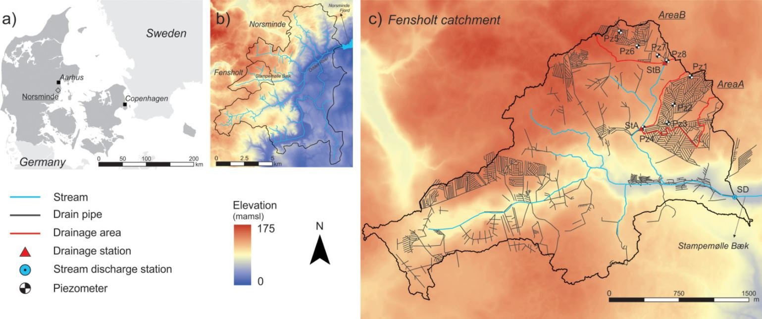
Fig. 1: Location of (a) the Norsminde catchment in Denmark (55°58′N, 10°08′E), (b) the Fensholt catchment within the Norsminde catchment, (c) a zoom-in on the Fensholt catchment showing topography (1.6 m digital elevation model), mapped drainage networks, drainage discharge measurement stations (StA and StB) with their respective drainage areas (AreaA and AreaB) and stream discharge station on the Stampemølle Bæk stream at the outlet of the catchment (SD). Eight observation piezometers are located in the two drainage areas (Pz1–Pz4 in AreaA and Pz5–Pz8 in AreaB).
This is a really interesting paper focused on modeling discharge from two tile drainage networks within the small agricultural Fensholt catchment in Denmark using HydroGeoSphere. One very interesting aspect of this study is the comparison made between model outputs produced by HydroGeoSphere and a previously constructed MIKE SHE model of the larger Norsminde catchment, which encompasses the primary study area for the HGS model presented here (Figure 1).

Fig. 2: 2-D mesh with refined nodes highlighted for both drainage areas, streams and topography areas where the surface slope is greater than 9%.
The HGS model in this study is a great example application of HGS for agricultural catchments, incorporating a mesh refined along two tile drain networks and the local stream network. The authors took special care to also refine the model mesh in areas of high vertical relief, specifically in areas with a surface slope >9% (Figure 2), resulting in a triangular element mesh with edge lengths ranging from 6 to 150 meters. In the subsurface domain the model was discretized vertically into a total of 18 layers to a depth of 20m. To better represent drainage dynamics, the first 3m of soil below ground surface were highly refined, with half of the available layers being applied in this shallow depth, with the highest refinement applied at the depth of the tile drain networks. The HGS model was forced using hourly disaggregated precipitation data, included a critical depth boundary at the catchment outlet, and incorporated a specified downward flux at the bottom of the model to account for deeper flow as the model was not bounded by a low-permeability geological unit.

Fig. 3: (a) Geological units in the heterogeneous stochastic best model, (b) vertical cross section through the model, and (c) a zoom on this section in the zone where drainage areas of interest are located. Top soil units cover the entire catchment from ground surface to 3 m deep. From 3 to 20 m deep (bottom of the model), units from a geological model created by He et al. [2014] are displayed. The vertical exaggeration for all figures is 10X.
While it is tempting to draw direct comparisons between HGS and MIKE SHE based on these models, it’s important to acknowledge the differences in scale and conceptualization between the two simulations. The MIKE SHE model for example was designed with a uniform grid with much coarser resolution (100m x 100m). Due to the coarse mesh, tile drainage BCs were applied uniformly to all cells in the drainage regions. The MIKE SHE model also had much less frequent output frequencies (daily, vs hourly output for the HGS model). Notwithstanding any shortcomings of the MIKE SHE model, both models were able to accurately reproduce the general flow dynamics of the catchment and of total drainage discharge. Nevertheless, the HydroGeoSphere simulations were able to produce more realistic outputs than MIKE SHE for several key variables such as the general groundwater flow dynamics around drainpipes. And it should also be noted that MIKE SHE did perform better than HydroGeoSphere in some ways, for example the intensity of drainage peaks produced by MIKE SHE were lower than HGS, and generally closer to the observed values. Then again, some of the observed peaks were not reproduced at all, by either simulation engine.
It's also interesting to note some of the shortcomings of the HydroGeoSphere model in this study (published over 6 years ago) and the ways that HydroGeoSphere has improved in the interim. The authors note that “[t]he drain node approach in HydroGeoSphere assumes that water entering the drains leaves the domain without being discharged in the subsurface domain or at land surface, which is generally observed in the field. […] Calibration against stream discharge was thus not feasible with HydroGeoSphere.” However, in recent years the “flux nodal from outlet” boundary condition was introduced to HydroGeoSphere, which would allow water removed from drainage nodes to be reinjected/discharged at a downstream location within the model.
Overall this is a very interesting study that highlights some of the key strengths and weaknesses of HydroGeoSphere and MIKE SHE, and provides a great case study in the use of HydroGeoSphere’s discrete tile drainage domain for simulating groundwater flow dynamics in an agricultural catchment with widespread subsurface drainage infrastructure.
“Nodes in HydroGeoSphere, along with finer mesh discretization, probably allowed for finer drainage flow simulation and enhanced lateral drainage flow, as seen with better peak flow simulated in HydroGeoSphere.”
Plain Language Summary:

Fig. 7: At the top, the topography is displayed in Fensholt and in the drainage areas of interest. (a, b) Pressure head distribution along vertical cross sections in AreaA is shown for the HeSB model (0.0–3.0 m depth, vertical exaggeration = 10) in May 2013. (c, d) Depth to water table is also shown for both AreaA and AreaB. Targeted output times were selected before a drainage peak (Figures 7a and 7c, 21 May 2013) and at maximum peak flow (Figures 7b and 7d, 23 May 2013).
In temperate regions, climate conditions may cause groundwater levels to be at or very close to the land surface, resulting in reduced crop yields. Therefore, a substantial part of agricultural lands is drained by subsurface pipes. While measuring drainage discharge is easy, identifying the origin of drainage water is complicated. This is where computer models are useful. Models allow for representing the underground of a selected region in numerical replicas. By building such replicas, we can virtually observe water flowing in the underground and at the land surface. Understanding the effect of drainage on water flow is essential to choose appropriate management techniques regarding fertilizer application by farmers for example. Yet reproducing drainage water flow with models is a challenge. In our case, we chose to build a replica of the Fensholt agricultural area in Denmark. Drainage outflow from two agricultural fields showed that the structure of the shallow underground, which is not thoroughly known, controls drainage outflow. This suggests that improving the underground knowledge is crucial to set effective farming strategies.
Abstract:
Seasonal variations of tile drainage discharge were simulated in the 6 km2 Fensholt catchment, Denmark, with the coupled surface and subsurface HydroGeoSphere model. The catchment subsurface is represented in the model by 3 m of topsoil and clay, underlain by a heterogeneous distribution of sand and clay units. Two subsurface drainage networks were represented as nodal sinks. The spatial distribution of the heterogeneous units was generated stochastically and their hydraulic properties were calibrated to reproduce drainage discharge for one network and verified with drainage discharge for the other network. Simulated discharge was compared to that of another model for which the heterogeneous sand and clay units were replaced by a homogeneous unit, whose hydraulic conductivity was the mean value of the heterogeneous model. With the homogeneous model, drainage dynamics were correctly simulated but drainage discharge was less accurate compared to the heterogeneous model. Simulated discharge was also compared to that of a larger-scale model created with the MIKE SHE code, built with the same heterogeneous model. HydroGeoSphere and MIKE SHE generated drainage discharge that was significantly different, with better simulated groundwater dynamics data produced by HydroGeoSphere. Nodal sinks in HydroGeoSphere reproduced drain flow peaks more accurately. Calibration against drainage discharge data suggests that drain flow is controlled primarily by geological heterogeneities included in the model and, to a lesser extent, by the nature of the soil units located between the drains and ground surface.
Want to read more about tile drains being used in HydroGeoSphere research? Click here!